CS-466/566: Math for AI

Module 01: MinMax Optimization

Dr. Mahmoud Mahmoud

The University of Alabama

2026-03-23

1. Motivation: Why Optimization?●

2. Derivatives: Measuring Change○

3. Gradient Ascent○

4. The Problem of Local Extrema○

5. From Maximization to Minimization (Gradient Descent)○

The Tax Revenue Problem

Imagine you’re elected prime minister. You want to maximize tax revenues.

If tax rate = 0% → Revenue = $0 (nothing collected)
If tax rate = 100% → Revenue ≈ $0 (nobody works)

The Sweet Spot: Somewhere between 0% and 100% lies the rate that maximizes revenue.

But where exactly?

Goal: Find $x^*$ such that $\qquad f(x^*) \ge f(x)\qquad$ for all $x$.

The Revenue Function

Your economists derive a revenue model:

import math
def revenue(tax):
    return 100 * (math.log(tax + 1) - (tax - 0.2)**2 + 0.04)

Do not worry about the exact form of the function, just know that it is a function that we want to maximize. It takes a single input, the tax rate, and returns the revenue.

Where Are We Now?

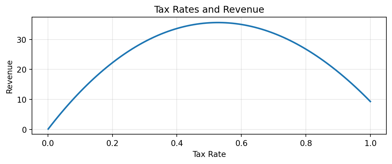
Your country currently has a 70% flat tax. Is this optimal?

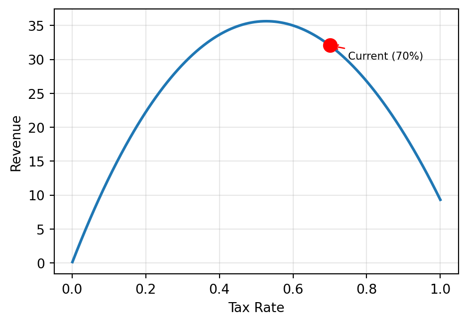
current_rate = 0.7

xs = np.linspace(0.001, 1, 500)
ys = [revenue(x) for x in xs]

fig, ax = plt.subplots(figsize=(5, 3.5))
ax.plot(xs, ys, linewidth=2)
ax.plot(current_rate,
        revenue(current_rate),
        'ro', markersize=10)
ax.annotate('Current (70%)',
    xy=(current_rate,
        revenue(current_rate)),
    xytext=(0.75, 30), fontsize=8,
    arrowprops=dict(arrowstyle='->',
                    color='red'))
ax.set_xlabel('Tax Rate')
ax.set_ylabel('Revenue')
ax.grid(True, alpha=0.3)
plt.tight_layout()
plt.show()

We need a precise answer — not just a guess from the plot!

1. Motivation: Why Optimization?✓

2. Derivatives: Measuring Change●

3. Gradient Ascent○

4. The Problem of Local Extrema○

5. From Maximization to Minimization (Gradient Descent)○

What is a Derivative?

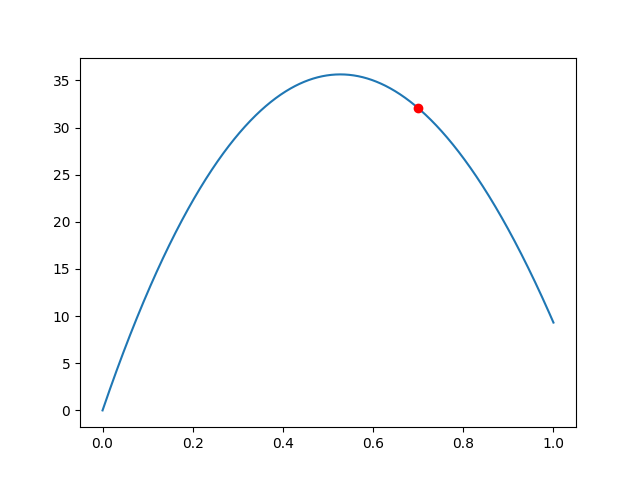
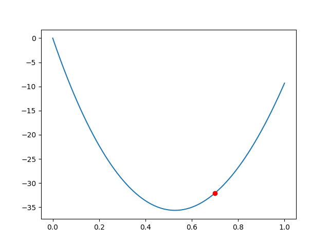
The derivative of $f$ at a point $x$ measures the slope of the tangent line:

\[f'(x) = \lim_{h \to 0} \frac{f(x+h) - f(x)}{h}\]

Interpretation:

$f'(x) > 0$: function is increasing → move right to go up
$f'(x) < 0$: function is decreasing → move left to go up
$f'(x) = 0$: critical point → possible maximum or minimum!

Numerical Approximation

When we can’t compute $f'(x)$ analytically, we approximate it:

Forward difference: $\frac{f(x+h) - f(x)}{h}$ — error is $O(h)$

Central difference: $\frac{f(x+h) - f(x-h)}{2h}$ — error is $O(h^2)$ ✅

Central difference is more accurate: it cancels first-order error terms.

Derivative of the Revenue Function

Our revenue function: $f(x) = 100\left[\ln(x+1) - (x-0.2)^2 + 0.04\right]$

Applying calculus rules:

\[f'(x) = 100\left[\frac{1}{x+1} - 2(x - 0.2)\right]\]

def revenue_derivative(tax):
    return 100 * (1/(tax + 1) - 2 * (tax - 0.2))

#> Derivative at current rate of 70%
print(f"f'(0.7) = {revenue_derivative(0.7):.2f}")

f'(0.7) = -41.18

$f'(0.7) < 0$ → revenue is decreasing at 70%. We should lower the tax rate!

What Does the Derivative Sign Tell Us?

Negative derivative at the red point:

→ Function is going downhill

→ To increase $f$, move left (decrease $x$)

Positive derivative at the red point:

→ Function is going uphill

→ To increase $f$, move right (increase $x$)

Taking a Step in the Right Direction

Since $f'(0.7) < 0$, we should decrease the tax rate.

Key idea: Move in the direction opposite to the negative derivative.

current_rate = 0.7
step_size = 0.003

#> Take one step: move opposite to negative derivative
current_rate = current_rate + step_size * revenue_derivative(current_rate)
print(f"New rate: {current_rate:.4f}")
print(f"New revenue: {revenue(current_rate):.2f}")

New rate: 0.5765
New revenue: 35.35

Revenue increased! Can we keep going?

1. Motivation: Why Optimization?✓

2. Derivatives: Measuring Change✓

3. Gradient Ascent●

4. The Problem of Local Extrema○

5. From Maximization to Minimization (Gradient Descent)○

The Gradient Ascent Update Rule

Repeat the step-taking process until convergence:

\[x_{\text{new}} = x_{\text{current}} + \alpha \cdot \nabla f(x_{\text{current}})\]

Where:

$\alpha$ = step size (learning rate) — controls how big each step is
$\nabla f(x)$ = gradient (derivative) — points in the direction of steepest ascent
If $\nabla f > 0 \quad$: move right (increase $x$)
If $\nabla f < 0 \quad$: move left (decrease $x$)

Intuition: Always walk uphill. Stop when the ground is flat ($\nabla f \approx 0$ ).

Gradient Ascent Algorithm

Step	Action
1	Choose initial $x_0$ and step size $\alpha$
2	Compute gradient $\nabla f(x_k)$
3	Update: $x_{k+1} = x_k + \alpha \cdot \nabla f(x_k)$
4	If $\|\alpha \cdot \nabla f\| < \text{threshold}$ → stop
5	Otherwise → go to Step 2

Stopping rule: When the change is smaller than a threshold, we’ve converged.

Gradient Ascent in Python

current_rate = 0.7
step_size = 0.003
threshold = 0.0001

for i in range(1000):
    rate_change = step_size * revenue_derivative(current_rate)
    current_rate = current_rate + rate_change

    if abs(rate_change) < threshold:
        print(f"Converged after {i+1} iterations")
        break

print(f"Optimal tax rate: {current_rate:.4f}")
print(f"Maximum revenue:  {revenue(current_rate):.2f}")

Converged after 7 iterations
Optimal tax rate: 0.5274
Maximum revenue:  35.64

Visualizing Gradient Ascent

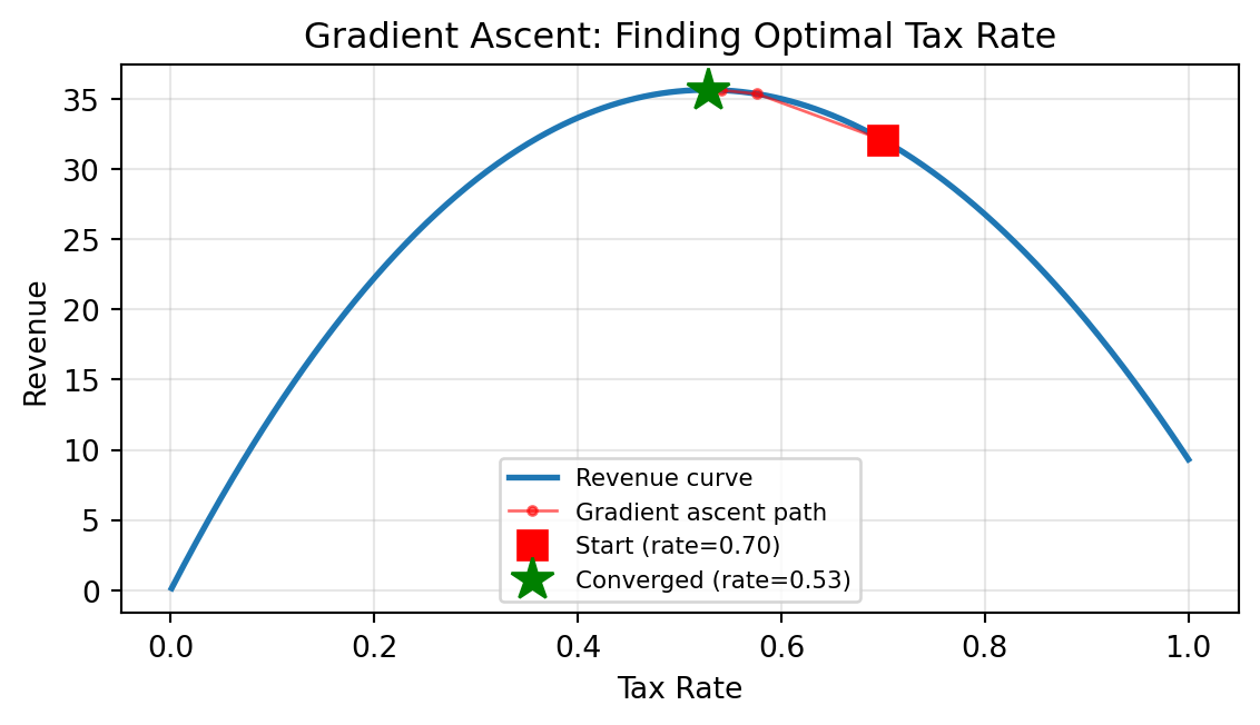
Starting from 70%, gradient ascent converges to the optimal tax rate in a few dozen steps.

1. Motivation: Why Optimization?✓

2. Derivatives: Measuring Change✓

3. Gradient Ascent✓

4. The Problem of Local Extrema●

5. From Maximization to Minimization (Gradient Descent)○

Local vs. Global Maximum

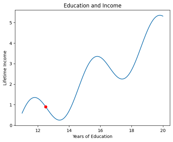
Gradient ascent finds a local maximum — the nearest peak.

But that may not be the global maximum!

The Problem:

Local Peak: Higher than immediate surroundings, but not the highest overall
Mountain Analogy: Climbing to a foothill summit — you’d need to go downhill first to find a taller peak
Gradient ascent never goes downhill → it can get stuck

No simple fix! This is a fundamental limitation of greedy local search.

Education and Income: A Real-World Analogy

The Trap of Local Optima:

Dropping out of school gives immediate income
But staying in school → higher long-term earnings
You must temporarily decrease income to reach the global maximum

Gradient ascent is greedy — it can’t see the bigger picture.

1. Motivation: Why Optimization?✓

2. Derivatives: Measuring Change✓

3. Gradient Ascent✓

4. The Problem of Local Extrema✓

5. From Maximization to Minimization (Gradient Descent)●

Gradient Descent: Flipping the Sign

In machine learning, we usually want to minimize a loss function, not maximize.

Two ways to switch:

Option 1: Negate the function then maximize negative of $f(x)$ instead

Option 2: Flip the update rule sign:

\[x_{\text{new}} = x_{\text{current}} \mathbin{\color{red}{-}} \alpha \cdot \nabla f(x_{\text{current}})\]

That’s it! One sign change turns gradient ascent into gradient descent.

This is the foundation of training neural networks.

Gradient Descent in Python

import numpy as np
import matplotlib.pyplot as plt

def f(x):
    return np.sin(5*x)*x + np.cos(2*x)*x + np.sin(15*x)

def numerical_derivative(func, a, h=0.0001):
    return (func(a + h) - func(a - h)) / (2 * h)

#> Gradient Descent
x_current = 1.0
alpha = 0.001
for i in range(1000):
    x_current = x_current - alpha * numerical_derivative(f, x_current)

print(f"Local minimum at x = {x_current:.4f}")
print(f"f(x) = {f(x_current):.4f}")

Local minimum at x = 1.1434
f(x) = -2.3557

Same algorithm, opposite direction. Gradient descent is the workhorse of modern AI.

Summary

Concept	Key Takeaway
Derivative	Measures slope — tells us which direction is “uphill”
Gradient Ascent	$x_{\text{new}} = x + \alpha \nabla f(x)\qquad$ — walk uphill to maximize
Local Extrema	Greedy search can get stuck — no guarantee of global optimum
Gradient Descent	$x_{\text{new}} = x - \alpha \nabla f(x) \qquad$ — walk downhill to minimize

Next up: Extending these ideas to multivariable functions and partial derivatives.

Thank You!

Step	Action
1	Choose initial \(x_0\) and step size \(\alpha\)
2	Compute gradient \(\nabla f(x_k)\)
3	Update: \(x_{k+1} = x_k + \alpha \cdot \nabla f(x_k)\)
4	If \(\|\alpha \cdot \nabla f\| < \text{threshold}\) → stop
5	Otherwise → go to Step 2

CS-466/566: Math for AI

TABLE OF CONTENTS

The Tax Revenue Problem

The Revenue Function

Where Are We Now?

TABLE OF CONTENTS

What is a Derivative?

Numerical Approximation

Derivative of the Revenue Function

What Does the Derivative Sign Tell Us?

Taking a Step in the Right Direction

TABLE OF CONTENTS

The Gradient Ascent Update Rule

Gradient Ascent Algorithm

Gradient Ascent in Python

Visualizing Gradient Ascent

TABLE OF CONTENTS

Local vs. Global Maximum

Education and Income: A Real-World Analogy

TABLE OF CONTENTS

Gradient Descent: Flipping the Sign

Gradient Descent in Python

Summary

Thank You!